My wiki | Site / MDTheory

Our simulations are large scale computational experiments that use simplifying assumptions to understand biological behavior on the molecular scale. While this provides many insights that are not possible with traditional in vivo tests, it is important to understand the methodology involved to recognize the limitations of this technique.

Modeling Atoms

In order to model molecules, we first have to decide on the best way to model atoms. In particular, atoms can be thought of as hard spheres or soft spheres. In the hard sphere model, atoms are like billiard balls, with no forces acting on them until they interact via collision. In the soft sphere mode, forces on atoms are a continuous function of distance. Soft sphere models are considered superior because atoms interact in ways other than collisions, such as via electrostatic attraction and repulsion.

Potential Energy Surface

Each possible arrangement of the atoms of the ribosome has a calculable potential energy that is the sum of the PE of each atom. If we imagine a smooth change in geometry, i.e. moving one atom through space at a time, we can map out an energy landscape (the potential energy surface - PES). In a system like the ribosome, which has many many atoms, there are many degrees of freedom. Using Cartesian x,y,z coordinates, the potential energy is a function of 3N points, where N is the number of atoms in the system. This quickly becomes difficult to visualize directly as one dimension is needed to visualize the energy, leaving only 1-2 dimensions to represent coordinates. This means that we need to take a slice of the actual multidimensional landscape. Practically, this means that usually we think of potential energy on the y-axis and some combination of spatial parameters on the x (and sometimes z)-axis(axes). All other degrees of freedom should be considered as allowed to vary, rather than being held fixed.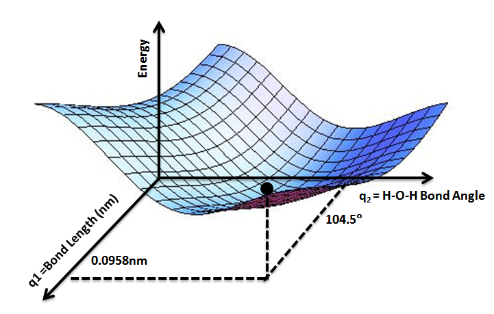

On such diagrams, we are most interested in finding energy minima (stable structures) and saddle points (transition structures). Note that a transition structure represents a point on the potential energy surface, not a point on the free energy landscape (analagous to a transition state). This means that other contributions to the free energy, such as entropic effects are not considered. The shape of the surface (e.g. the flatness and width at the bottom of a well) is also useful, as it tells us about the relative population of a similar set of structures.

Force Fields

One way we could generate the PES would be to do quantum mechanical (QM) calculations, however this would be extraordinarily expensive computationally. In order to get around this QM is used to come up with force field parameters that can be applied to molecules so electrons can be ignored. This is sometimes called molecular mechanics (MM).

The potential energy surface can be represented mathematically. The computed energy can be thought of as the sum of bonded interactions (strain from bond length, angle, or torsion) and non-bonded interactions (van der Waals and electrostatic) at a certain set of atomic positions.

For bonded atoms, the ideal bond conditions will vary by the atoms involved (e.g. the ideal geometry of a carbon atom will be different for a sp3 hybridized carbon, a sp2 hybridized carbon, a carbocation, and a carbon in a ring of size n), with each case defined as a different atom type. A force field can be defined as a collection of atom types, the functions used to compute their potential energy/degree of strain, and constants used in the functions. While a larger number of atom types will more closely approximate chemical reality, for every atom type added, force field constants and ideal geometries between that atom and every other atom type must be generated. These parameters come from a mixture of experimental data and QM calculations.

Bond strain and bond angle can be modeled with Hooke's Law, which produces a parabola that models the well in an energy curve. The limitation here is that for large bond distances, the bond doesn't continue to become higher energy, it levels off until the bond breaks. The Morse potential best models the energy when two atoms are bonded, but because we don't usually sample bonds far from their equilibrium distance Hooke's Law works just as well and is much simpler to use in calculations. Additionally, neglecting bond breakage and formation is one reason why many force fields cannot model reactive chemistry. Use of Hooke's Law also means that the calculations are most accurate when the system is in a lower-energy state.

Torsional strain is modeled as a periodic function with respect to improper dihedral angle (the angle between two planes created by 3 of 4 atoms bonded in series) using a Fourier series.

For atoms that are not bonded but are still close in space, there are no bond stretching, bond angle, or torsional parameters. Instead, if the interaction is non-polar, we consider weakly attractive van der Waals forces (arising from transient dipoles) at long distances and repulsive overlap forces at short distances. This is modeled with the Lennard-Jones potential. If the interaction is polar, we consider electrostatic forces (opposite charges attract and like charges repel). This is modeled with Coulomb's law. To calculate the electrostatic term, imagine pairwise calculations are made between every atom in the system. This would be the most accurate approach, however it would take a long time! Instead, an 8-12A cutoff is used for the pairwise calculations and everything beyond this range is modeled with Ewald summation, a mean electric field. The atoms to include in these calculations are determined by maintaining a neighbor list that is updated periodically after a certain number of time steps. Further, we assume that the interaction energy is the sum of two-body contributions.

So far, we can see some of the essential first steps in molecular modeling: assign atom types to all atoms in the system, define what is bonded together (which linkages have strain that needs to be calculated), and look up all the force constants and equilibrium values for the different contributors to the overall potential energy.

Energy Minimization

Once we are able to calculate the potential energy of a particular conformation, we begin with an initial geometry (e.g. from a PDB) and adjust atomic positions to minimize that energy to the nearest local minimum. Two important assumptions are made at this point: that the initial structure we use is sufficiently similar to the native structure, and that the native structure is close to a significant energy minimum. One method used to in energy minimization is steepest descent, which moves downhill on the PES at right angles. This technique is better when the initial conformation is farther from the minimum geometry and can be thought of as coarse adjustment. Another method used is conjugate gradient, which moves downhill on the PES at a calculated angle. This converges on the minimum geometry more quickly than steepest descent when the structure is already close to minimized and can be thought of as fine adjustment.

Simulations

Two major types of simulation are Monte Carlo (MC) and Molecular Dynamics (MD).

Monte Carlo simulations generate a population of geometries that are probabilistically weighted by temperature. A method called simulated annealing is often used. This technique makes a stochastic (random) adjustment to the current coordinates and recalculates the overall energy of the system. It is only dependent on the immediately previous step, making it a Markov chain method. If the new coordinates are better, they are accepted. If the new coordinates are worse, they are accepted with a probability related to the "temperature" of the system (at higher temperatures, an unfavorable move is more likely). The system begins at high temperature, making it more likely to accept energetically unfavorable moves. This allows exploration of the PES rather than being stuck in a well. Over time, the "temperature" of the system is decreased, with the goal of falling into the global minimum. Note that there is no concept of time in this type of simulation, as only one atom is moved at a time, making it impossible to make measurements of time-dependent properties.

In Molecular Dynamics simulations, some initial geometry and set of velocities define a starting condition. Initial heating of the system distributes velocities to atoms based on the Maxwell-Boltzmann law. Each next step is determined by calculating the force on each atom (equation above), and therefore the acceleration (from F = ma). As the simulation moves forward one step in time, the Newtonian equations of motion are used to update the xyz coordinates, making MD deterministic. Because the total energy of the system is conserved, the ergodic hypothesis states that the trajectories should sample the PES in an energy-weighted way. However, because some wells may be too high in energy to be thermally accessible, it is possible that not all wells are sampled using this technique. A method called quenched dynamics is often used to find energy minima. This technique starts at high temperature, allowing a simulation to roam over the high energy region of the PES and then is cooled so that the simulation falls into a minimum. Because atomic positions and velocities are updated at every time step, MD simulations are appropriate for measuring time-dependent properties.

In calculating the PES, we use the Born-Oppenheimer approximation to justify only considering nuclear positions. Because nuclei are so massive compared to electrons, the energy of a molecule in the ground electronic state can be considered a function of nuclear coordinates. As a result, nuclei are treated classically (as definitive positions) and electrons are treated with quantum mechanics (as probability distributions). In MD, the phase space, the collection of geometries of the system over time, is characterized by the momentum and position of each atomic nucleus. If the timestep (the amount of time between calculations) is too large, the positions are changing too much and the trajectory is deviating from the determined phase space, which can lead to unrealistic energies and the resulting forces causing the system to blow apart.

Solvent and Surface Area

In order to accurately model molecular behavior, our systems are solvated. There are two main techniques used for solvation: implicit solvent models and explicit solvent models. Implicit solvent models replace individual solvent molecules with a continuous medium. A dielectric constant is used to handle solvent electrostatics and another set of parameters (proportional to the SASA - see below) is used to handle non-electrostatic solvent effects such as cavitation, dispersion, and structural changes. This has the benefit of not making the simulated system any larger, saving computational resources. However, important interactions between the solvent and solute would be missed. Explicit solvent, on the other hand, involves simulation of individual solvent molecules. Waters are placed around the molecule in a lattice and then assigned velocities, allowing them to melt. This introduces many water molecules into the simulations, which can become computationally expensive. Ideally, we do not want to waste a lot of time calculating the properties of bulk solvent, so we would like the box that our molecule is in to be as small as possible. However, the system will move around during the simulation and interact with the edges of the box, which can lead to unintended effects. To get around this, we apply periodic boundary conditions. Essentially, we surround a central cell containing the solvated system with images of itself. This makes the system "feel" like it is in bulk solvent without having to simulate a large number of water molecules.

The explicit solvent model that we use is TIP3P, which is a simple model with rigid molecular geometry. It provides three sites for electrostatic interactions (the oxygen and two hydrogens) and the van der Waals interactions are centered on the oxygen.

One useful measurement to monitor in order to understand the behavior of a system is the contact surface. To measure this, a probe (usually 1.4A -- the size of a water molecule) is traced over the surface of a molecule. If the re-entrant surface is measured, the output is the surface area that the probe is excluded from. If the solvent accessible surface area (SASA) is measured, the output is the area traced by the center point of the probe as it rolls over the surface of the molecule.

Additional Resources

Computational Chemistry Lectures - UMN (02.01 to 02.08 - PES and Force Fields, 06.01 to 06.07 - Solvent Models)

Molecular Modelling: Principles and Applications (A. R. Leach)

Molecular Dynamics Simulation: Elementary Methods (J. M. Haile)